7.2 Measuring Risk
We are to make a decision as to the best choice of two investment options, Investment Portfolio Option A and Investment Portfolio Option B —— on the basis of an objective assessment of their yearly Returns over the past 20 years. The frequency of the yearly Returns on investments in each of the Investment Portfolio Options is given in the following Distribution Tables.
|
Investment Portfolio Option A Frequency Distribution of Return of x% p.a. over |
Probability of achieving this (Probability Distribution) |
||
|
Return (x% p.a.) |
Frequency (years) |
||
|
2% |
3 |
0.15 |
|
|
4% |
4 |
0.2 |
|
|
6% |
3 |
0.15 |
|
|
10% |
4 |
0.2 |
|
|
12% |
3 |
0.15 |
|
|
26% |
2 |
0.1 |
|
|
30% |
1 |
0.05 |
|
|
Frequency Distribution of Return of x% p.a. over |
Probability of achieving this (Probability Distribution) |
||
|
Return (y% p.a.) |
Frequency (years) |
||
|
7.8% |
3 |
0.15 |
|
|
9% |
4 |
0.2 |
|
|
9.4% |
3 |
0.15 |
|
|
10% |
4 |
0.15 |
|
|
10.8% |
3 |
0.15 |
|
|
11.8% |
2 |
0.15 |
|
|
12.6% |
1 |
0.05 |
|
The Yearly Returns from which the above Frequency Distributions have been calculated are set out in the following Tables. (We will be using these Yearly Returns below to plot the scatter of the Returns achieved over the 20 year period.)
|
|
Investment Portfolio Option B |
|||
|
Year |
Return (% p.a.) |
Year |
Return (% p.a.) |
|
|
1 |
10 |
1 |
7.8 |
|
|
2 |
4 |
2 |
10.8 |
|
|
3 |
26 |
3 |
9 |
|
|
4 |
2 |
4 |
11.8 |
|
|
5 |
12 |
5 |
10 |
|
|
6 |
4 |
6 |
7.8 |
|
|
7 |
10 |
7 |
10.8 |
|
|
8 |
2 |
8 |
9.4 |
|
|
9 |
6 |
9 |
11.8 |
|
|
10 |
30 |
10 |
9.4 |
|
|
11 |
10 |
11 |
10 |
|
|
12 |
12 |
12 |
9 |
|
|
13 |
26 |
13 |
11.8 |
|
|
14 |
6 |
14 |
10 |
|
|
15 |
4 |
15 |
12.6 |
|
|
16 |
2 |
16 |
9 |
|
|
17 |
10 |
17 |
10.8 |
|
|
18 |
6 |
18 |
9.4 |
|
|
19 |
4 |
19 |
7.8 |
|
|
20 |
12 |
20 |
9 |
|
Using formula (F9), we compute our Expected Return from Investment Portfolio Option A as follows :
| Expected return | = | E (x) | = |
n Σi = 1 |
PRi Xi |
= (0.15 x 2%) + (0.2 x 4%) + (0.15 x 6%) + (0.2 x 10%) + (0.15 x 12%)
+ (0.1 x 26%) + (0.05 x 30%)
= 9.9% p.a.
Again, using Formula (F9), we compute our Expected Return from Investment Portfolio Option B as follows :
| Expected return | = | E (y) | = |
n Σi = 1 |
PRi yi |
=(0.15 x 7.8%) + (0.2 x 9%) + (0.15 x 9.4%) + (0.15 x 10%) + (0.15 x 10.8%)
+ (0.15 x 11.8%) + (0.05 x 12.6%)
=9.9% p.a.
The Expected Return from each of the two Investment Portfolio Options is equal at 9.9% p.a.
So which Investment Option should we choose?
Common sense would dictate that we choose the Investment Option that carries the smaller Risk.
We should therefore choose the Investment Option that we would expect to have the smaller deviation from the Expected Return of 9.9% p.a.
---------------
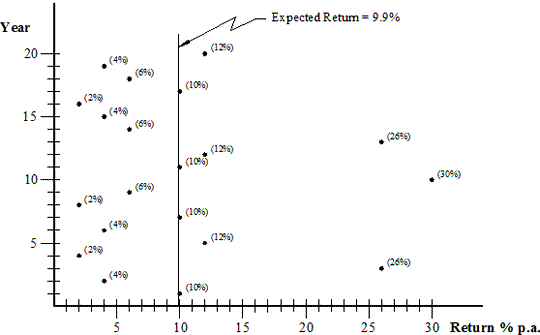
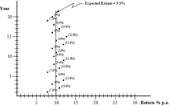
A plot of the Returns achieved by each Investment Option for each year over the past 20 years (see the diagrams below) clearly shows the dispersion of Returns about the Expected Return of 9.9% p.a. These diagrams show the scatter of the Returns achieved over the past 20 years (they have been plotted using the Yearly Returns data tabulated above).
It is obvious that investment in Investment Portfolio Option B is much less Risky than investment in Investment Portfolio Option A.
The Dispersion of the Return Values around the Expected Return Value of 9.9% p.a. is much less scattered in the case of Investment Portfolio Option B than in the case of Investment Portfolio Option A.
Based on the past performance data for Investment Portfolio Options A and B, we would expect that the Risk, as measured by the deviation from the Expected Return of 9.9% p.a., would be much smaller in the case of Option B than in the case of Option A. However, we have no objective comparison measure of the Risk associated with each of the Investment Options.
---------------
As a measure of the Risk associated with a particular Investment Option, we use the Statistics measurement for the Standard Deviation (σ). The Standard Deviation (σ) measures the dispersion of the various possible outcomes, in this case percentage returns, about the Expected Return.
The Standard Deviation (σ) is computed from the Statistics measurement for Variance (σ2) .

Investment Portfolio Option A

Investment Portfolio Option B
If there are n possible outcomes, each with a separate value xi and a corresponding probability of occurrence PRi for i = 1 to n, then the Expected Value of x is given by the formula :
| E (x) | = |
n Σi = 1 |
PRi Xi | (i.e. (F9)) |
and the Expected Value of  x - E (x)
 2, called the Variance σ2(x) of the probability distribution of the various values of x, is given by the formula :
| (F10) | σ2(x) | = | E  x - E (x) x - E (x) 2 2 |
| = |
n Σi = 1 |
PRi  Xi - E (x) Xi - E (x) 2 2 |
Note! Don’t be intimidated by these formulae! The Examples that follow will make their use and meaning clear.
The Standard Deviation σ(x) is the square root of the Variance σ2(x).
Note! The Standard Deviation σ(x) is measured in this way, i.e. as the square root of the Variance σ2(x), because by computing the Variance first we eliminate the negative sign for values of  x - E (x)
  where E(x) is greater than x. The Expected Value of
  x - E (x)
  is zero. This, the accepted convention by which Risk is measured, comes from the conventional 'Statistics' comparative measure for 'dispersion', and has been in use since long before the advent of computers. (See the boxed NOTE! below.)
So, for Investment Portfolio Option A, the Variance σA2 is computed as follows:
| σ2(x) | = |
n Σi = 1 |
PRi  Xi - E (x) Xi - E (x) 2 2 |
| σA2 | = | 0.15 ( 2 – 9.9 ) 2 + 0.2 ( 4 – 9.9 ) 2 + 0.15 ( 6 – 9.9 ) 2 + 0.2 ( 10 – 9.9 ) 2 + 0.15 ( 12 – 9.9 ) 2 + 0.1 ( 26 – 9.9 ) 2 + 0.05 ( 30 – 9.9 ) 2 |
| = | 65.39 (% p.a.) 2 |
Because the Variance is measured in ‘ percentage per annum ’ squared, the dispersion measurement is more clearly understood in terms of the Standard Deviation σ (x), this being measured in ‘percentage per annum’.
| σ(x) | = | √σ2 (X) | |||
| σA(x) | = | √ 65.39 | = | 8.09% p.a. |
For Investment Portfolio Option B, the Variance σB2 is computed as
| σ2(x) | = |
n Σi = 1 |
PRi  Xi - E (x) Xi - E (x) 2 2 |
| σB2 | = | 0.15 ( 7.8 – 9.9 )2 + 0.2 ( 9 – 9.9 )2 + 0.15 ( 9.4 – 9.9 )2 + 0.15 ( 10 – 9.9 )2 + 0.15 ( 10.8 – 9.9 )2 + 0.15 ( 11.8 – 9.9 )2 + 0.05 ( 12.6 – 9.9 )2 |
| = | 1.89 (% p.a.)2 |
and the Standard Deviation σB(x) =1.37% p.a.
---------------
It can be seen from the above that, while both Investment Portfolio Option A and Investment Portfolio Option B offer the same Expected Return of 9.9% p.a., the indicative measurement of the extent to which the Actual Returns deviate from the Expected Return (i.e. the indicative measurement of the Dispersion), as measured by the Standard Deviation (σ) , clearly shows that investment in Investment Portfolio Option A is far MORE RISKY than investment in Investment Portfolio Option B.
σA is much greater than σB
---------------
We now have an objective comparison measure of the Risk associated with each of the Investment Options —— the Standard Deviation.
It is, however, worth noting that the computation of the Expected Value of | x – E (x) |, where | x – E (x) | is ‘The Absolute Value’ of the Difference between each outcome value and the Expected Value, yields the exact expected deviation measurement. (The absolute Value eliminates the negative sign after computation of the Difference between each outcome value and the Expected Value, {x – E (x)}.
For example:
In the case of Investment Portfolio Option A, the expected deviation measurement is:
0.15 | 2 – 9.9 | + 0.2 | 4 – 9.9 | + 0.15 | 6 – 9.9 | + 0.2 | 10 – 9.9 | +
0.15 | 12 – 9.9 | + 0.10 | 26 – 9.9 | + 0.05 | 30 – 9.9 | = 5.9 % p.a.
In the case of Investment Portfolio Option B, the expected deviation measurement is:
0.15 | 7.8 – 9.9 | + 0.2 | 9 – 9.9 | + 0.15 | 9.4 – 9.9 | + 0.15 | 10 – 9.9 | +
0.15 | 10.8 – 9.9 | + 0.15 | 11.8 – 9.9 | + 0.05 | 12.6 – 9.9 | = 1.14 % p.a.
