If we invest an equal amount  R  at the End of each period for a duration of  n  interest periods, at an interest rate  i  per interest period, these investments will yield a Final Sum  S  at the end of the  n  periods.

The formulae expressing the relationship between the parameters involved in this investment situation are referred to as Uniform Series Payment Formulae and are as follows:

(F3)S=R

(F4)R=S

                                                       ---------------


The following diagrammatic illustration will facilitate your understanding of the inter-relationship between the Uniform Series Payment Formulae parameters.

(For an understanding of the derivation of these formulae see Appendix 5/2.)

Uniform (i.e. equal in amount) Series of Payments (R)

i = interest rate per
interest period

                                                  Final Sum (S) achieved

 

---

In the above Uniform Series of Payments investment situation we see, from Formula (F3), that we can realise a Final Sum  S  at the end of  n  interest periods, by investing an equal amount  R  at the End of each interest period (over the  n  periods) at an interest rate  i  per interest period.

But from Formula (F1) (see Section 5.1) we know that a Final Sum  S, at the end of  n  interest periods, can also be realised by investing a present sum  P (at Time Zero) at an interest  i  per interest period, over the  n  periods.

i.e. S   =   P(1 + i)n

Hence the following formulae:

(F5)R=P

(F6)P=R

The superposition (below), of the diagrammatic illustration of the investment situation for a Single Payment above that for a Uniform Series of Payments, will facilitate your understanding of the inter-relationship between Uniform Series Payment Formulae and Single Payment Formulae ——— to achieve the same Final Sum (S). 

---

 

 

Single Payment / Investment (P)
at Time Zero

                                                                  Final Sum (S) achieved

---

It is important to understand that financial analysis evaluation using these basic Uniform Series Payment Formulae is on the basis that the series of equal payments are End of interest period payments. The mathematics of the financial analysis evaluation using these basic formulae is on the basis that the first payment / investment is made at the End of the first interest period.

For example: ——— if the interest period applicable is 1 month, then the first payment / investment is to be made at the end of the first month, and Time Zero will therefore be at the beginning of the first month; ——— if the interest period applicable is 1 year, then the first payment / investment is to be made at the end of the first year, and Time Zero will therefore be at the beginning of the first year.

Note!  For situations where payments are made from the start of the first interest period (which is generally the case with investments), the use of the general Geometric Series format would be employed (as in the derivation of the Uniform Series Payment Formulae in Appendix 5/2) or a time-value adjustment could be made to the above formulae. But these situations are not of relevance to the subject matter of this website-book.  

We will now illustrate the use and meaning of the Uniform Series Payment Formulae, by example. 

---

 

 

Example 5.3

If we invest an equal amount (R) of £2,000 at the end of each year for 5 years, at an interest rate of 10% p.a., what will be the Final Value (FV) of our investment at the end of the 5 year period?

From Formula (F3)S=R

R = £2,000n = 5 yearsi = 10% p.a.

ThereforeS=£2,000

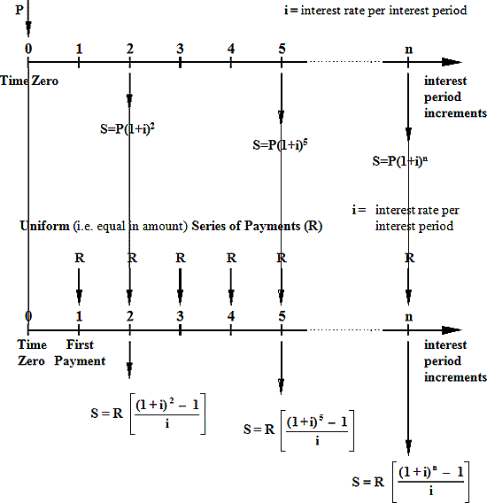
S=£2,000 =£12,210.20

i.e. the Final Value of our investment at the end of the 5 year period will be £12,210.20.

Let us now use this example to check our Uniform Series Formulae.

We tabulate the investment sequence over the five year period as follows: 

Interest rate  i = 10% p.a.
Year	Value at start of year	Value at end of year plus end of year investment R (R = £2,000)
1	Nil	£2,000
2	£2,000	(£2,000 x 1.1) + £2,000
3	£4,200	(£4,200 x 1.1) + £2,000
4	£6,620	(£6,620 x 1.1) + £2,000
5	£9,282	(£9,282 x 1.1) + £2,000

 

So, our Final Value (FV) at the end of year 5 is ( £9,282 x 1.1 ) + £2,000 = £12,210.20, as we have already computed using the Uniform Series Formula (F3).

---

 

Using the parameters of Formulae (F1), (F2), (F3), (F4), (F5) and (F6), and the data of Example 5.3 above, the following logically equivalent statements can be made:

1.	The Present Value (PV) of a Future Sum (S) of £12,210.20 that we will receive in 5 years time, where the cost of money over the time period is 10% p.a., is £7,581.57. P== ==£7,581.57

NOTE!  Remember that the Present Value (PV) is the value at TIME ZERO. 

2.	The Present Value (PV) of a Uniform Series of receipts (i.e. an Annuity) (R) of £2,000 that we will receive at the end of each year over a 5 year period, where the interest rate payable is 10% p.a., is also £7581.57 P=R =£2,000 =£2,000 =£7,581.57

3.	If we borrow a Present Sum (P) of £7,581.57 at an interest rate of 10% p.a. and we are to repay this loan over 5 years by repaying equal instalments at the end of each year, then our Uniform Annual Series of Repayments (R) will be £2,000 per year at the end of each of the five years. From Formula(F5)R=           P R=£7,581.57 =£2,000
4.	If we borrow a Present Sum (P) of £7,581.57 at an interest rate of 10% p.a. and we repay this loan by repaying £2,000 (R) at the end of each year, then our loan will be fully repaid at the end of exactly 5 years. R=P                                           £2,000      =        £7,581.57

 

We know from the above Example that the value of  n  computes at 5 years.

NOTE !  In the above case the value of n could be computed directly, using logarithms. (For the mathematical purists, this logarithmic solution method, using the parameters of Example 5.3 above, is illustrated in Appendix 5/2.) But, again, a main purpose of these early Examples is to introduce the mathematical Iteration process of ‘trial and error’ by which an unknown parameter can be computed.

5.	If we borrow a Present Sum (P) of £7,581.57 and we repay this loan by repaying £2,000 (R) at the end of each year for a period of 5 years, then we will have been charged an interest rate of 10% p.a. on our loan. R          =          P £2,000=£7,581.57

 

Again —— from the above Example —— we know that the value of  i  computes at 10% p.a.; but if we did not already know the value of  i, we would have to work it out by Iteration.

Note! If we borrow a Present Sum (P), as in a Repayment Mortgage, over  n  interest periods at an interest rate  i  per interest period, we repay the loan by repaying equal amounts  R  at the end of each of the interest periods.

6.

If we invest an equal amount of £2,000 (R) at the end of each year for a period 5 years and we receive a Final Sum (S) of £12,210.20 at the end of the 5 year period, then we will have achieved an (Internal) Rate of Return of 10% p.a. on our investment.                                S                    =                            R                           £12,210.20=£2,000

 

Again — from the above Example — we know that the value of  i  that makes this expression valid is 10% p.a.; but if we did not already know the value of  i, we would have to work it out by Iteration.

We will now illustrate the process of Iteration for computing (Internal) Rate of Return, by example.

---

Example 5.4

 

If we invest £3,000 at the end of each year for a period of 5 years and we receive a Final Sum of £19,518.13 at the end of the 5 year investment period, what (Internal) Rate of Return will we have achieved on our investment?

We know:R=£3,000

n=5 years

S=£19,518.13

i=?

We therefore use the formula (F3)

                               S             =              R

                         i.e. £19,518.13=£3,000

We want to compute the value for  i  that makes this expression valid.

We first assume a trial value for  i.

Let  i = 10% p.a. Hence Trial No. 1.

The process of Iteration is tabulated as follows: 

Trial No.	Equal Amount End of year Investment R = £3,000	Trial value of i	Computed value of	Corresponding Final Sum S = £3,000
1	£3,000	10%	6.1051	£18,315.30
2	£3,000	15%	6.742381	£20,227.14
3	£3,000	13.143%	6.498688	£19,496.06
4	£3,000	13.2%	6.506043	£19,518.13

From Trial No. 1,i = 10% p.a. yields  S = £18,315.30. This is lower than the Final Value of £19,518.13 required, so we must try a higher value of  i.

From Trial No. 2,i = 15% p.a. yields  S = £20,227.14. This is higher than the Final Value of £19,518.13 required, so we must try a lower value of  i.

We now know that the value of  i  lies between 10% p.a. and 15% p.a.

We can speed up our process of Iteration by using a linear approximation, for the values of  i  versus the corresponding values of  S, between the values already computed for  i  at 10% p.a. and 15% p.a.

Trial No. 1  i1=10%p.a. yields  S1=£18,315.30

Trial No. 2  i2=15%p.a. yields  S2=£20,227.14

Interpolating linearly between these values we compute a trial value for  i3  that corresponds to an  S3  value of £19,518.13

This Interpollation for  i3  is done thus:  
                                                  
                                  i = 10% +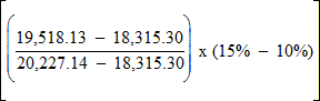

                                     i = 10% +        =  13.143%

Hence Trial No. 3 at  i3 = 13.143%

This yields  S3 = £19,496.06

If the relationship between  i  and  S  had been exactly linear, then our trial value of i  at 13.143% would have yielded  S  at £19,518.13, and not £19,496.06. However, you can see that an approximation to a linear relationship brings us much closer to the true value of  i ; it speeds up the Iteration process.

A continuation of this process of Iteration, using linear interpolation between the values already computed, will result in the value of  i  being computed at 13.2% p.a. ——— i.e. the (Internal) Rate of Return on our investment is 13.2% p.a.